Introduction to Machine Learning
Arthur Samuel defines ML as “the field of study that gives computers the ability to learn without being explicitly programmed.”
Tom Mitchell defines ML as “[a] computer program is said to learn from experience E with respect to some class of tasks T and performance measure P, if its performance at tasks in T, as measured by P, improves with experience E.”
Example: playing checkers.
T = the task of playing checkers.
E = the experience of playing many games of checkers against itself
P = the percent of games won in the world tournament.
The goal of any Machine Learning problem as stated in the given definition is to improve the performance over some task given enough experience. The components of a ML problem are stated above; the first step in formulating a problem is to define the target function, what exactly do you want the model to learn. Next comes characterizing the experience for the model, which is a set of data that is separated into a training set and a testing set. In the context of Supervised Learning where the correct answer or desired label is also supplied with the data point. The chosen model is fed <X, Y> value pairs from the training set, and then evaluated on the test set. The performance measure is how well the model learned the target function. This is indicated by how well the model can generalize during the testing phase.
Selecting a Target Function
This step is a major design choice, the Target Function determines exactly what type of knowledge will be learned and how this will be used by the by performance program. How the function is represented involves weighing tradeoffs. On one hand, we wish to choose a very expressive model (the type of learning algorithm), which determines what type of things that can be learned. The more expressive and complex the model, the more complex tasks that can be learned. The tradeoff is that more data is needed to train more complex models.

"The more features you try to learn, the more data you need"
Unsupervised Learning
You are given a dataset but do not have an idea of what the output will be. In some cases relationships are determined to “cluster” variables together. In other cases, unsupervised learning is used to separate things in a chaotic environment.
Clustering Example: Taking a list of NBA player data and stats and grouping players that do similar things together. Non-Clustering Example: Take a recording of people speaking and isolating the individual voices.
Supervised Learning
You are given a data set and already know what our correct output should look like, getting a sense of the relationship between the output and input. Essential, you are given the “the right answers”.
There are two kinds of supervised learning problems REGRESSION & CLASSIFICATION. Regression is trying to determining the results in a continuous output. Classification is outputting inputs into categories.
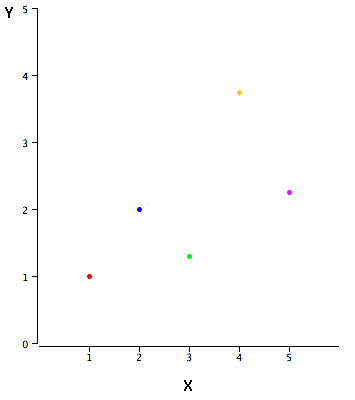
In simple linear regression, we predict scores on one variable from the scores on a second variable. The variable we are predicting is called the criterion variable and is referred to as Y. The variable we are basing our predictions on is called the predictor variable and is referred to as X. When there is only one predictor variable, the prediction method is called simple regression. In simple linear regression, the topic of this section, the predictions of Y when plotted as a function of X form a straight line. The example data in Table 1 are plotted in Figure 1. You can see that there is a positive relationship between X and Y. If you were going to predict Y from X, the higher the value of X, the higher your prediction of Y.
| X | Y |
|---|---|
| 1.00 | 1.00 |
| 2.00 | 2.00 |
| 3.00 | 1.30 |
| 4.00 | 3.75 |
| 5.00 | 2.25 |
The error of prediction for a point is the value of the point minus the predicted value (the value on the line). Table 2 shows the predicted values (Y') and the errors of prediction (Y-Y'). For example, the first point has a Y of 1.00 and a predicted Y (called Y') of 1.21. Therefore, its error of prediction is -0.21.
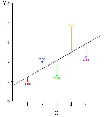
| X | Y | Y' | Y-Y' | (Y-Y')2 |
|---|---|---|---|---|
| 1.00 | 1.00 | 1.210 | -0.210 | 0.044 |
| 2.00 | 2.00 | 1.635 | 0.365 | 0.133 |
| 3.00 | 1.30 | 2.060 | -0.760 | 0.578 |
| 4.00 | 3.75 | 2.485 | 1.265 | 1.600 |
| 5.00 | 2.25 | 2.910 | -0.660 | 0.436 |
You may have noticed that we did not specify what is meant by "best-fitting line." By far, the most commonly-used criterion for the best-fitting line is the line that minimizes the sum of the squared errors of prediction. That is the criterion that was used to find the line in Figure 2. The last column in Table 2 shows the squared errors of prediction. The sum of the squared errors of prediction shown in Table 2 is lower than it would be for any other regression line. The formula for a regression line is Y' = bX + A
where Y' is the predicted score, b is the slope of the line, and A is the Y intercept. The equation for the line in Figure 2 is Y' = 0.425X + 0.785
For X = 1, Y' = (0.425)(1) + 0.785 = 1.21.
For X = 2, Y' = (0.425)(2) + 0.785 = 1.64.