The traditional pencil drawing algorithm uses a texture background image to simulate the effect of a pencil repeatedly drawing on the paper to produce texture, without taking into account the difference of textures in different areas of the image, and can only generate images of a fixed style. But in real life, artists draw pencil drawings styles are varied. Considering that the convolutional neural network has a good effect on image texture feature extraction, it can simulate inconsistent textures and has a certain similarity with biological vision. I present the method to optimize the single generation result of traditional pencil drawing algorithms based on a Deep Neural Network.

It uses the convolutional neural network to extract the features of the artist's hand-drawn pencil drawings and uses the Adam optimization algorithm to optimize the results to obtain the algorithm of the pencil drawing image so that the generated pencil drawing retains the original details and information. It makes more flexibility in the style of the final result image. After generating the texture image, it is combined with traditional algorithms to generate the final results

The problem we're trying to solve using Neural Style Transfer and geometric models is to create sketches that mimic many styles of an artist.

Before we detect the edges, we must notice that minor noises on the picture could actually affect the final output image. Thus, the implementation above may produce a lot of artifacts. We can solve this problem by using median filtering. After removing these noises, we calculate the original image use this formula. $$ G = \sqrt{((\delta_x)^2+(\delta_y)^2)} $$ The detection effect of this formula is very weak. I think the $Lu^{[1]}$ may not use the modified formula in the real sense, because this step has a great influence on the final effect. I have adopted some other edge detection algorithms that can better detect the effect, like Sobel. But in the end, I use the original formula.

Because the result has too much noise and the edge does not continue, the author performs the convolution in 8 directions on the obtained results, the convolution kernel is 1 along the specified direction, and the other values are 0 (in fact, considering the anti-aliasing problem, the convolution kernel is obtained by bilinear interpolation), The size of the convolution kernel is proposed to be 1/30 of the width or height of the image (I think this is a bit unacceptable, when it is too large, there will be obvious unreasonable lines), the formula is : $$ G_i =\varphi_i*G $$ The operation is rotate the kernel by 22.5 degrees and convolution with edge map. In fact, the convolution is the motion blur according to the specified angle.

After obtaining the convolution results in all directions, for each pixel, the response of the direction with the largest convolution value is set to G, and the response of other directions is set to 0. The formula is $$ C_i(p)=\left{ \begin{aligned} &G(p)\ \ &if\ argmax_i{G_i(p)}=i\ &0\ \ &otherwise \end{aligned} \right. $$

After that, we again perform directional convolution on the resulting responses for each aspect use this formula. $$ S'=\sum_{i=1}^{8}(\varphi_i\otimes C_i) $$ This is a example for this step

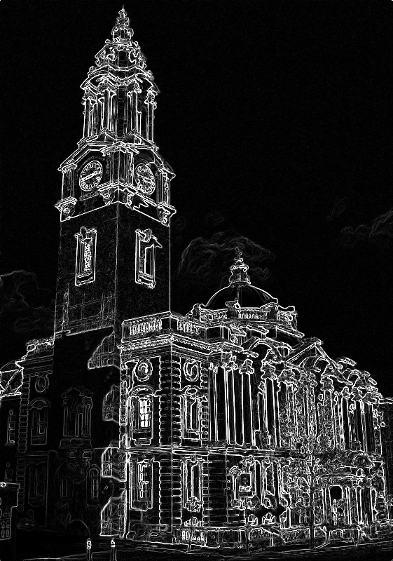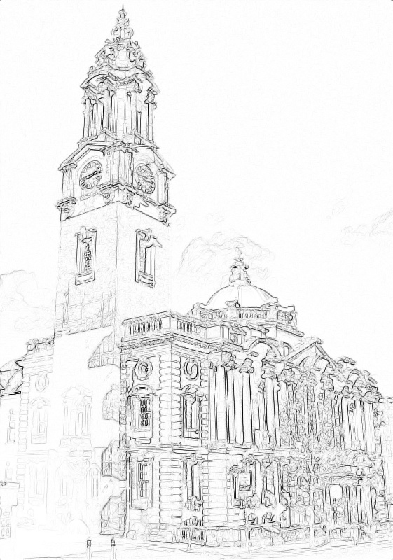The gradient map	The stroke map

According to the observation and analysis of a large number of hand-drawn pencil drawing image data, the distribution of histograms is very different from the images we captured, but they all form a certain rule, which can be expressed by a certain empirical formula. Therefore, we can set a fixed histogram and then map the image's own histogram to this histogram as the result.

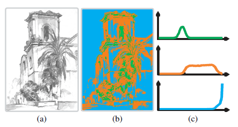
In the below image, (a) is a hand-drawn pencil drawing, (b) is a hard-divided image of shadows, mid-tones, and highlights, and (c) corresponds to the histogram distribution of shadows, mid-tones, and highlights, respectively. It can be seen that the shadows are basically normally distributed, the mid-tones are roughly evenly distributed, and the highlights are Laplace distribution. Therefore, the author constructs three functions for each of the three parts to simulate the curve.

In the pencil drawings drawn by hand, since the paper is generally white, the proportion of highlights must actually be very large. This is reflected in the histogram that the distribution curve is steeper when it is close to level 255. The authors propose the following function as the distribution curve for this part. $$ p_1(v)=\left{ \begin{aligned} &\frac{1}{\sigma_b}e^{-\frac{1-y}{\sigma_b}}\ &if\ v\leq1\ &0\ \ &otherwise \end{aligned} \right. $$

Simulate with a horizontally distributed line $$ p_2(\nu)=\left{ \begin{aligned} &\frac{1}{u_b-u_a}\ &if\ u_a\leq \nu\leq u_b\ &0\ \ &otherwise \end{aligned} \right. $$

The shadows part shows the change of image depth, which is simulated by a Gaussian curve $$ p_3(\nu)=\frac{1}{\sqrt{2\pi\sigma_d}}e^{-\frac{(\nu-\mu)^2}{2\sigma_d^2}} $$ These formula has different weights for different pencil drawings, so the author proposes a comprehensive formula to obtain the histogram corresponding to the final pencil drawing $$ p(\nu)=\frac{1}{Z}\sum_{i=1}^3\omega_ip_i(\nu) $$ According to different needs, different weight coefficients can be adjusted to achieve different mixing effects.

Based on experience, Lu proposes a set of data

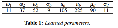
In this project, we use [25 40 18]

After we get this data, then we can do Histogram matching use MATLAB function histeq

This is a example for this step

In the $Neural-Style\ algorithm^{3},$ it define two distances, one for the content and one for the style. measures how different the content is between two images while measures how different the style is between two images. Then, we take a third image, the input, and transform it to minimize both its content-distance with the content-image and its style-distance with the style-image. Now we can import the necessary packages and begin the neural transfer.

In this algorithm, we only define the the style, and define the third image, the input, is a black noise image.

The style loss will act as a transparent layer in a network that computes the style loss of that layer. In order to calculate the style loss, we need to compute the gram matrix. A gram matrix is the result of multiplying a given matrix by its transposed matrix. In this application the given matrix is a reshaped version of the feature maps of a layer.

The feature map is reshaped to form a K x K matrix, where K is the number of feature maps at layer L and N is the length of any vectorized feature map.

Finally, the gram matrix must be normalized by dividing each element by the total number of elements in the matrix. This normalization is to counteract the fact that matrices with a large N dimension yield larger values in the Gram matrix. These larger values will cause the first layers (before pooling layers) to have a larger impact during the gradient descent. Style features tend to be in the deeper layers of the network so this normalization step is crucial.

We import a pre-trained neural network from ImageNet. We will use a 16 layer VGG network. We choose the serval layer to get the style feature map. In order to get the better result, we use the Adam optimizer, and pass our image to it.

For each iteration of the networks, it is fed an updated input and computes new losses. We will dynamically compute their gradients for each loss module. The optimizer reevaluates the module and returns the loss.

After 500 iteration, the gradients is down.

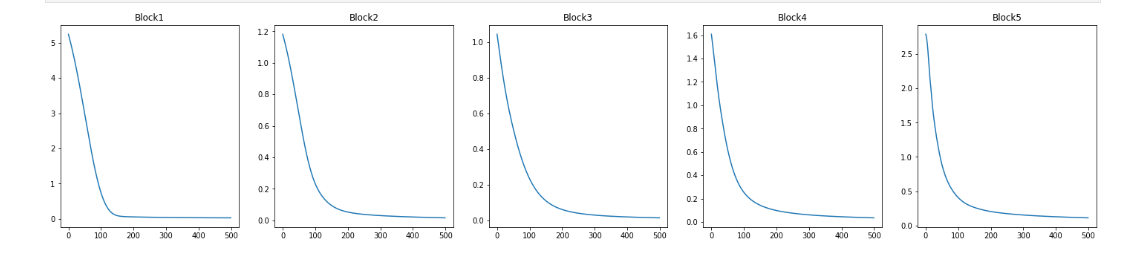
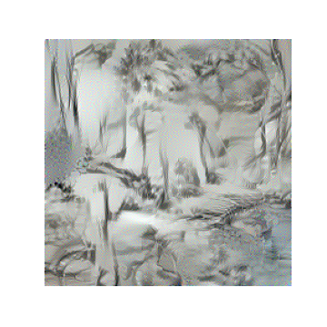
After all the iteration, we can get the final style map for the pencil texture. We need to cropped it to speed the calculate.

This is a example for this step

The pencil drawing by hand	After 2000 iterations	the cropped result

This is a pencil texture rendering use pencil texture and tone map.

The base idea is solve a equation. $$ \beta^*=argmin_\beta||\beta lnH-lnJ||_2^2+\lambda||\bigtriangledown \beta||^2_2 $$ This is a example for this step

We combine the pencil stroke S and tonal texture T by multiplying the stroke and texture values for each pixel to accentuate important contours, expressed as $$ R =S \cdot T $$ The final result is

$CycleGAN^{[2]}$ is another famous technique for image translation. The normal GAN architecture is a two-model approach in which the generator tries to produce images of the target domain while the discriminator tries to predict the authenticity of those generated images. CycleGAN is an extension of GAN which uses two generators and two discriminators. One generator tries to produce images of domain A while the other generator tries to produce images of domain B. Two discriminators try to predict whether images are from domain A or B respectively. One application of CycleGAN is image style transfer.

I also use CycleGAN to generate the pencil drawing image, but the result is not good.

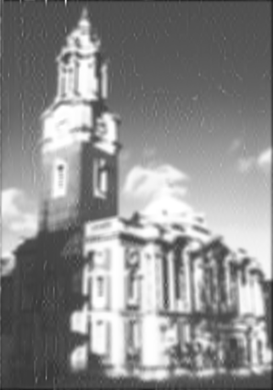
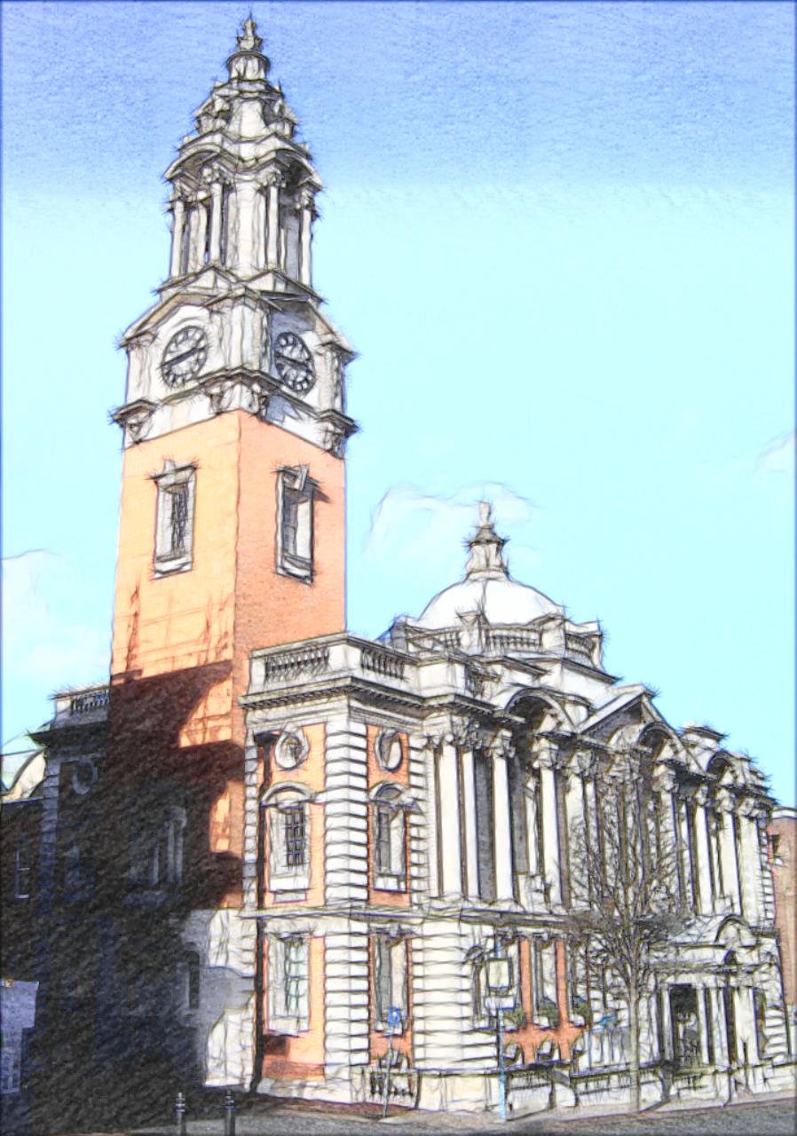
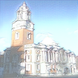
The input image	The paper result	The CycleGAN result	My result

We can clearly see that in the results of Lu and CycleGAN, the sky has obvious faults, and there is obvious overexposure. But Lu handles the details better than my results, due to the different styles of pencil texture.

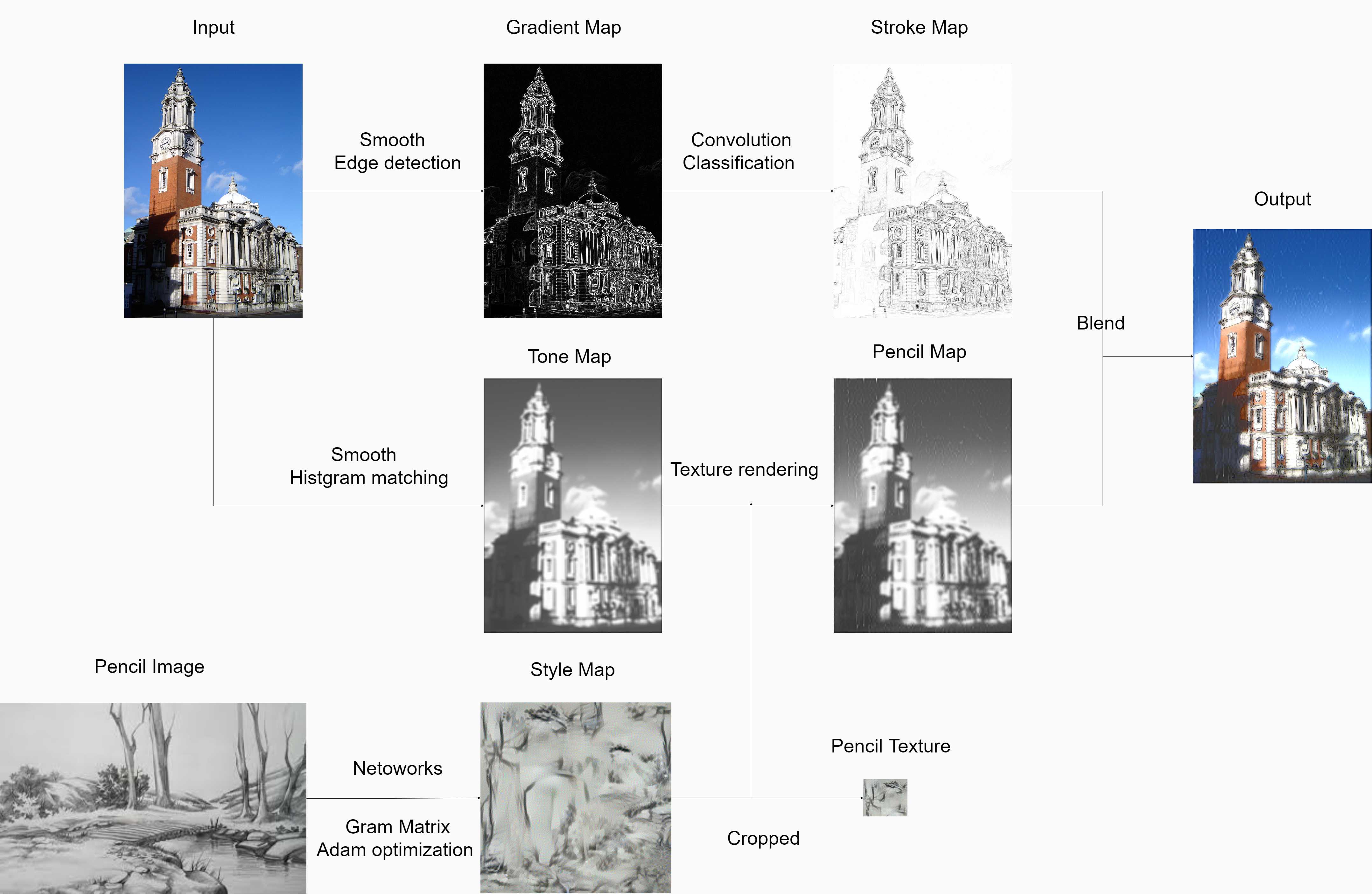
In this project, we implement an enhanced pencil drawing algorithm using Convolutional Neural Networks. First we try to create the Stroke Map and Tone Map. And we use the part of Neural Style Transfer algorithm to extracted the style map from a shallow layer. And combine the style map and tone map. Finally, we blend the Stroke Map and Pencil Map.

In the end, considering all aspects including the training time, we conclude that using Neural Style Transfer and geometric models outperforms the CycleGAN method.

[1] Combining Sketch and Tone for Pencil Drawing Production Cewu Lu, Li Xu, Jiaya Jia International ymposium on Non-Photorealistic Animation and Rendering (NPAR 2012), June, 2012

[2] Unpaired Image-to-Image Translation using Cycle-Consistent Adversarial Networks. Jun-Yan Zhu*, Taesung Park*, Phillip Isola, Alexei A. Efros. In ICCV 2017

[3] A neural algorithm of artistic style,L. A. Gatys, A. S. Ecker, and M. Bethge, 02-Sep-2015.

[4] https://pytorch.org/tutorials/advanced/neural_style_tutorial.html#style-loss

[5] https://github.com/ariG23498/NeuralStyleTransfer